Nonlinear Fiber Labby optocpo Run a simulationSimulate
Free · runs in your browser · nothing to install

Simulate how light reshapes itself inside an optical fiber.

A research-grade solver for nonlinear pulse propagation. Pick an example, move the sliders, and watch solitons break up, spectra explode into a supercontinuum, and pulses shift colour, all computed on our server in seconds.

9ready-to-run examples
4published results reproduced
< 0.2 %photon-number error per run
~20 stypical run on our server

Background: spectral evolution of the Dudley et al. (2006) supercontinuum benchmark, computed with this solver. Wavelength left to right, fiber length bottom to top.

01 · Simulator

Choose an example and press run

Our free server sleeps when idle, so the very first run after a quiet spell can take up to a minute. After that, runs take seconds and repeated settings are instant.

Loading examples…

Results will appear here.
02 · Validation

Checked against the literature

A simulator is only useful if you can trust it. These examples recreate published experiments and simulations; each card shows our own computed result, and you can rerun it yourself.

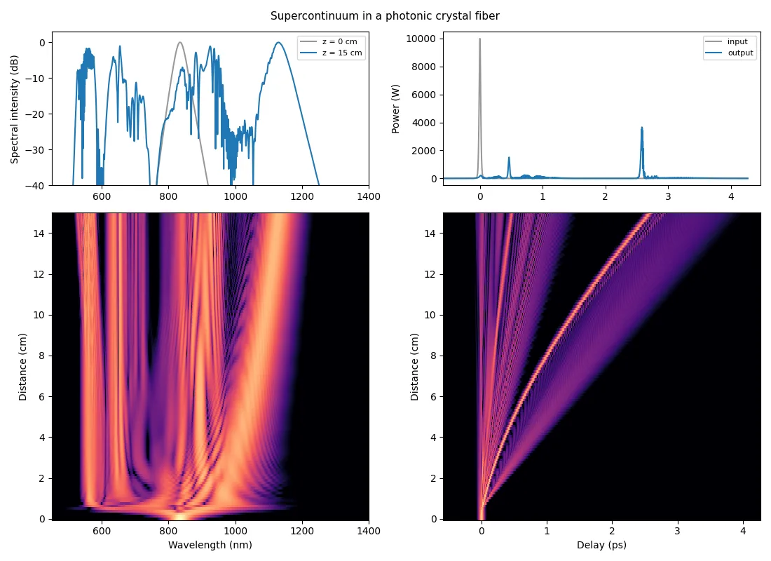
Computed supercontinuum evolution in a photonic crystal fiber: spectrum and temporal power versus distance
Dudley, Genty & Coen · Rev. Mod. Phys. 78, 1135 (2006) · Fig. 3

The supercontinuum benchmark

A 28 fs, 10 kW pulse at 835 nm in 15 cm of photonic crystal fiber. The soliton fissions within the first centimetre; a Raman soliton walks to the red while dispersive waves form in the blue.

output 514 – 1251 nm at −40 dB Run this example →
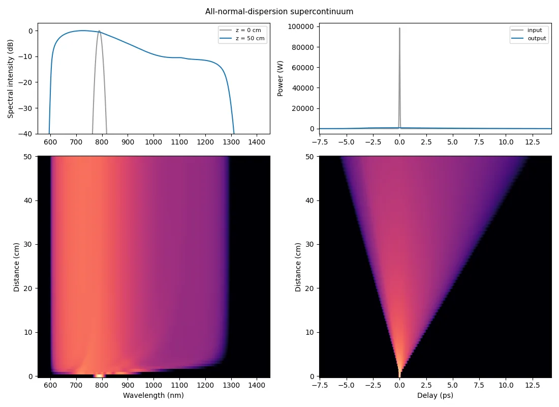
Computed all-normal-dispersion supercontinuum: smooth spectral broadening versus distance
Heidt et al. · Opt. Express 19, 3775 (2011) · Fig. 3

Coherent, flat supercontinuum

An all-normal-dispersion fiber pumped at 790 nm with 8 nJ. No solitons form: self-phase modulation and optical wave breaking give a smooth, coherent spectrum.

output 596 – 1312 nm at −40 dB Run this example →
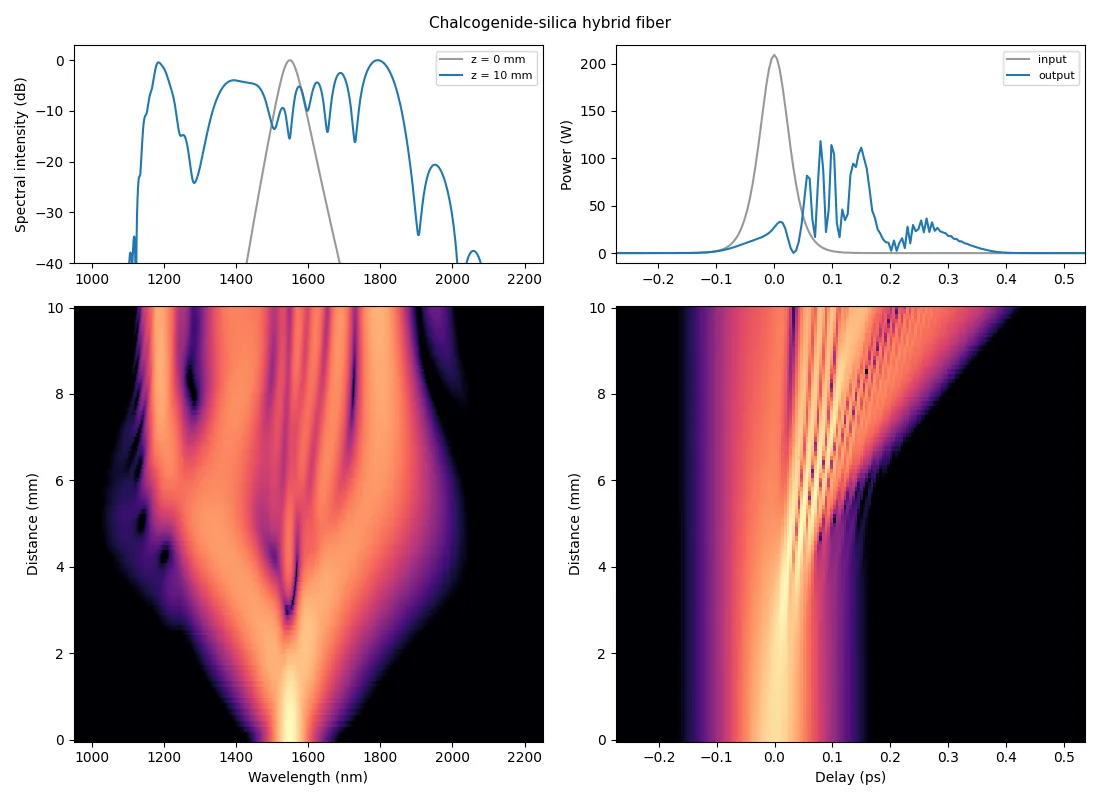
Computed supercontinuum in a chalcogenide-silica hybrid fiber pumped at 1550 nm
Granzow et al. · Opt. Express 19, 21003 (2011) · Fig. 4

Towards the mid-infrared

A chalcogenide-glass core inside silica, pumped at 1550 nm just above its 1513 nm zero-dispersion wavelength. The high nonlinearity pushes the spectrum beyond 2 µm.

output 1104 – 2078 nm at −40 dB Run this example →
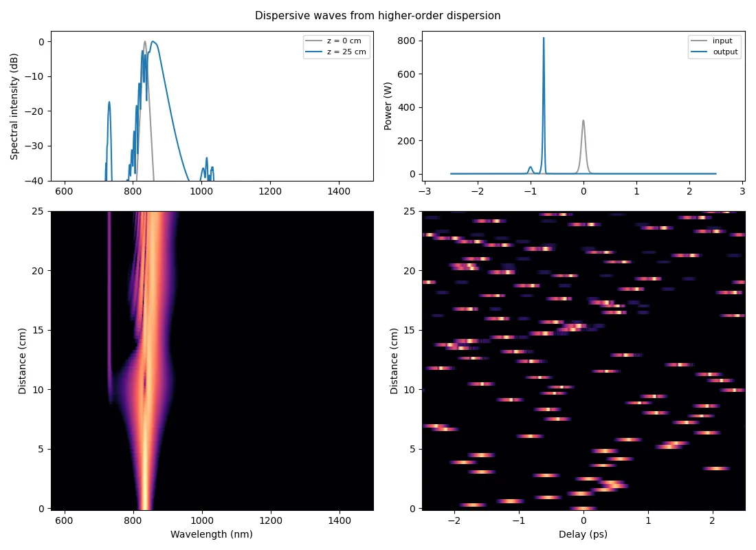
Computed dispersive-wave generation from a second-order soliton with higher-order dispersion
Roy, Bhadra & Agrawal · Opt. Lett. 34, 2072 (2009) · Fig. 1

Dispersive waves on demand

A second-order soliton with third-, fourth- and fifth-order dispersion. Changing the dispersion terms decides whether the soliton radiates in the blue, the red, or both.

dispersive waves at 734 nm and 1038 nm Run this example →
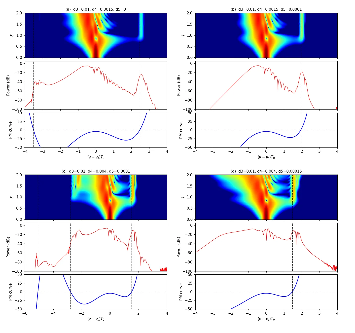
Four-panel reproduction of Roy et al. 2009 Fig. 1: spectral evolution, output spectra and phase-matching curves for four dispersion settings
Deep dive

Radiation lands where theory says it should

For each of the four dispersion settings in Roy et al., the top panel shows the computed spectral evolution, the middle the output spectrum, and the bottom the phase-matching curve between the soliton and linear waves.

The dashed lines mark where that curve crosses zero. The spectral peaks of the emitted dispersive waves fall on those lines, an independent check that the solver gets the physics, not just the picture, right.

0.004 – 0.18 %Photon-number error across all nine examples. Every run reports this conservation check in its results table, so you can judge each result yourself.
03 · Physics

What the solver computes

Every run integrates the generalized nonlinear Schrödinger equation, the standard model for ultrashort pulses in fibers and waveguides, with full dispersion and a delayed Raman response.

Generalized nonlinear Schrödinger equation ∂A∂z − ∑k≥2 ik+1k! βk ∂kA∂Tk = iγ (1+iτshock∂∂T) [A(z,T)∫R(T′)|A(z,T−T′)|2dT′]
dispersion

Any dispersion profile

Taylor coefficients to any order or a full tabulated β(ω), so measured fiber data and engineered waveguides go in directly.

nonlinearity

Kerr, self-steepening, Raman

Instantaneous Kerr effect, frequency-dependent γ(ω) with self-steepening, and a delayed Raman response for silica or chalcogenide glass.

raman models

Choice of Raman response

Blow–Wood silica, the Lin–Agrawal model with boson peak, As₂S₃ chalcogenide, or an instantaneous response to switch Raman off.

accuracy

Adaptive step-size control

A split-step integrator estimates its own local error at each step and adjusts the step length to keep it below a set tolerance, from gentle propagation to soliton fission.

geometry

Tapers and varying fibers

Dispersion and nonlinearity can change along the fiber from mode tables, with a correction that keeps photon number conserved through a taper.

diagnostics

Physics you can check

Spectral and temporal evolution maps, output spectrograms, spectral width, peak power, pulse width, energy and photon-number conservation for every run.

04 · Learn

Nonlinear fiber optics in six ideas

Short explanations of what you see in the simulator. Each one links to an example you can run and modify.

01

Dispersion

Different colours travel at different speeds. In the normal regime red light is faster than blue; in the anomalous regime it is the other way round. The group-velocity dispersion β₂ sets the dispersion length.

LD = T₀² / |β₂|See dispersion at work →
02

Solitons

With anomalous dispersion, the Kerr effect can exactly cancel dispersive spreading. The soliton number N compares the two; an N-th order soliton breathes and recovers every soliton period z₀ = (π/2) LD.

N² = γP₀T₀² / |β₂|Run a higher-order soliton →
03

Soliton fission

Perturbations such as higher-order dispersion and Raman scattering break a higher-order soliton into N fundamental solitons after roughly LD/N. This is the engine of most supercontinuum sources.

Lfiss ≈ LD / NWatch a soliton fission →
04

Raman self-frequency shift

Intrapulse Raman scattering transfers energy from the blue to the red side of a soliton's own spectrum, so the soliton continuously moves to longer wavelengths. Shorter pulses shift much faster, roughly as T₀⁻⁴.

dω/dz ∝ −T₀⁻⁴See a Raman soliton →
05

Dispersive waves

Near a zero-dispersion wavelength, a soliton can phase-match to linear waves on the other side of it and shed energy there as a narrow spectral peak, sometimes called optical Cherenkov radiation.

β(ω) − β(ωs) − β₁(ω − ωs) ≈ γPs/2Generate dispersive waves →
06

Normal-dispersion supercontinuum

In all-normal-dispersion fibers no solitons form. Self-phase modulation broadens the pulse and optical wave breaking fills in the spectrum, giving smooth, highly coherent continua for imaging and pulse compression.

coherent · flat · soliton-freeRun an ANDi fiber →
05 · Work with us

Need more than the examples?

The public lab uses fixed fibers and short runs. The full solver handles your own fibers, waveguides and parameter studies.

Software

Solver licence

The complete Python solver on your own machine, without the limits of the public lab.

  • Your own dispersion data, mode tables and tapers
  • Long fibers, fine grids and parameter sweeps
  • Run simulations from AI assistants through MCP integration
Ask about a licence
Consulting

Custom simulation studies

We model your design question and deliver figures, data and a written summary.

  • Supercontinuum and few-cycle source design
  • Fiber and taper dispersion engineering
  • Pulse compression and reproduction of published results
Describe your project
Education

Training and workshops

Hands-on nonlinear fiber optics for research groups, companies and courses.

  • Fundamentals with live simulations
  • From textbook cases to real fibers
  • Course material built on the lab examples
Plan a session
06 · FAQ

Questions

Is the Nonlinear Fiber Lab free?

Yes. All examples run free of charge. To keep the service available to everyone, parameters are limited to short runs and there is a fair-use limit on new runs per hour.

Where do the simulations run?

On our server. Your browser sends the example and parameter values and receives the figures and numbers back. Nothing is installed on your computer.

How accurate are the results?

The solver reproduces the spectral features of published results, including Dudley et al. (2006), Heidt et al. (2011), Granzow et al. (2011) and Roy et al. (2009). Every run also reports photon-number conservation, typically within 0.2 %.

Can I use the figures in a report or publication?

Yes. Please credit “Nonlinear Fiber Lab, optocpo (lab.optocpo.com)”.

Why did my first run take so long?

The lab runs on a free server that sleeps after a period without visitors. Waking it up takes up to a minute; after that, runs take seconds, and settings someone has already run are returned instantly.

Can I simulate my own fiber or waveguide?

The public examples use fixed fibers. For your own dispersion data, geometries or longer runs, contact us about a solver licence or a custom simulation study.